Convolution Methods¶

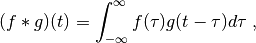
The convolution integral in one dimension is defined as

$(f*g)(t)=\int_{-\infty}^{\infty}f(\tau)g(t-\tau)d\tau\; ,$

and the discrete equivalent (which implies uniformly discretized data and kernel)

$(f*g)[n]=\sum_{m=-\infty}^{\infty}f[m]g[n-m] .$

Often both f and g often have some kind of symmetry around 0; openConv deals mainly with both f and g having some kind of symmetry. In the examples some more details are discussed and mentioned; in general the examples are a good way to learn how to understand and use the code.

import openConv
convObj = oc.Conv(nData, symData, kern, kernFun, symKern, stepSize, nResult, method = method, order = order)
result = convObj.execute(data)

Direct Convolution / Trapezoidal Rule¶

It is fairly common to use directly the discrete convolution to approximate the convolution integral, often with smaller improvements like using trapezoidal rule instead of rectangle rule. Especially relevant in case both f and g are smooth functions, this yields usually neither good order of convergence (second order with trapezoidal rule), nor fast calculation (quadratic O(N^2) computational complexity).

Direct convolution is chosen by setting method=0.

FFT Convolution¶

One option to get a faster calculation is instead of direct calculation is use of the Fast Fourier Transform (FFT) based convolution, or often called “fast convolution” algorithm. This approach gives linearithmic O(Nlog(N)) computational complexity, but possibly large relative and unpredictable errors of the result, since the error scales with the maximum value of the result. In case of functions with high dynamic range, e.g. exponential functions, the tails of the results are poorly resolved.

FFT convolution is chosen by setting method=1.

Fast Multipole Method with Chebyshev Interpolation¶

Even better computational complexity (linear O(N)) can be achieved by the Fast Multipole Method (FMM). There are so called black box FMM described in literature (e.g. by Tausch), which in principle work well for smooth kernels with not too high dynamic range.

FMM convolution is chosen by setting method=2.

Fast Multipole Method with Chebyshev Interpolation for Approximately Exponential Functions¶

In openConv we extend the FMM to functions with asymptotic somewhat exponential decay and thus can deal with a large class of functions with high dynamic range.

FMMEXP is chosen by setting method=3.

End Corrections¶

To increase the order of convergence openConv uses end corrections for the trapezoidal rule as described in the reference by Kapur. These end corrections can be used together with every convolution method by setting the keyword order to the desired order. If data points outside of the integration interval can be provided these end corrections are arbitrary order stable. Otherwise it is not recommended to go higher than 5th order. As of now we provide the coefficients up to 20th order. The Mathematica notebook which calculated these coefficients can be found in this repository as well.