example000_exponential
This is a simple example which calculates the convolution of a Gaussian with a symmetric approximately exponential kernel.
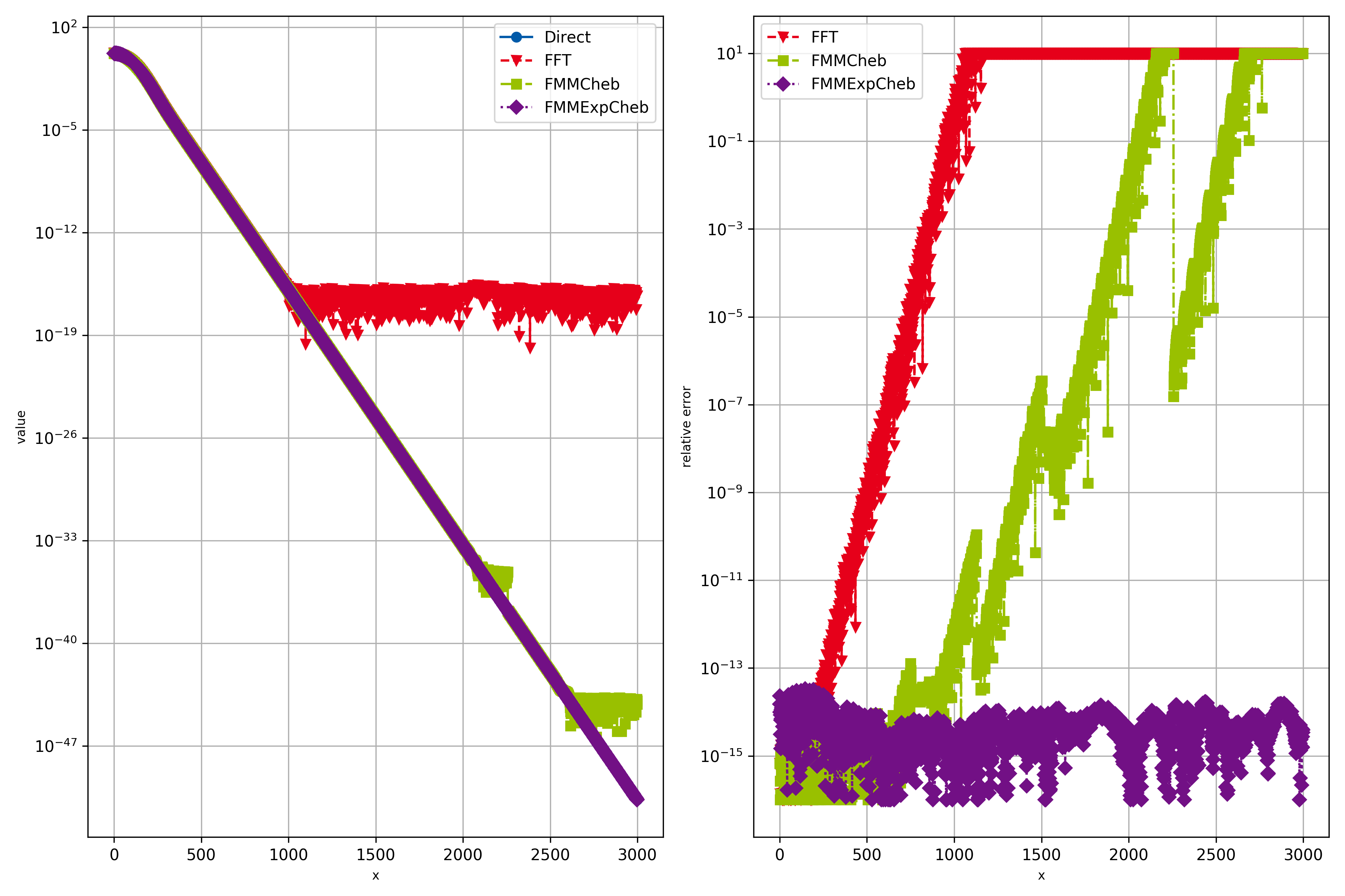
Simple convolution with somewhat exponential kernel.
1 2 3 4 5 6 7 8 9 10 11 12 13 14 15 16 17 18 19 20 21 22 23 24 25 26 27 28 29 30 31 32 33 34 35 36 37 38 39 40 41 42 43 44 45 46 47 48 49 50 51 52 53 54 55 56 57 58 59 60 61 62 63 64 65 66 67 68 69 70 71 72 73 74 75 76 77 78 79 80 81 82 83 84 85 86 87 88 89 90 91 92 93 94 95 96 97 98 99 100 | ############################################################################################################################################
# Simple example which calculates the convolution of two somewhat exponential functions.
# Results are compared with the direct solution. Mostly default parameters are used.
############################################################################################################################################
import openConv as oc
import numpy as np
import matplotlib.pyplot as mpl
############################################################################################################################################
# Plotting setup
params = {
'axes.labelsize': 8,
'font.size': 8,
'legend.fontsize': 10,
'xtick.labelsize': 10,
'ytick.labelsize': 10,
'text.usetex': False,
'figure.figsize': [12., 8.]
}
mpl.rcParams.update(params)
# Color scheme
colors = ['#005AA9','#E6001A','#99C000','#721085','#EC6500','#009D81','#A60084','#0083CC','#F5A300','#C9D400','#FDCA00']
# Plot markers
markers = ["o", "v" , "s", "D", "p", "*", "h", "+", "^", "x"]
# Line styles
linestyles = ['-', '--', '-.', ':','-', '--', '-.', ':','-', '--', '-.', ':']
lw = 2
fig, ((ax1), (ax2)) = mpl.subplots(1, 2)
############################################################################################################################################
# Parameters and input data
order = 5
orderM1Half = max(int((order-1)/2),0)
nData = 1000
xMaxData = 8.
sigData = 0.5
stepSize = xMaxData/(nData-1)
xData = np.linspace(-orderM1Half*stepSize, orderM1Half*stepSize+xMaxData, nData+2*orderM1Half)
data = np.exp(-0.5*xData**2/sigData**2) # data can actually be arbitrary
# Kernel
lamKernel = 0.2
def kern(xx):
return np.exp(-xx/lamKernel) + 10.*np.exp(-3.*xx/lamKernel)
nKernel = 2000
# Parameters and output result
nResult = nData+nKernel-1 # Can be chosen arbitrary, but use typical length for example
xResult = np.linspace(0., (nResult-1)*stepSize, nResult)
xKernel = np.linspace(0., (nResult+nData-2)*stepSize, nResult+nData-1)
kernel = kern(xKernel)
############################################################################################################################################
# Create convolution object, which does all precomputation possible without knowing the exact
# data. This way it's much faster if repeated convolutions with the same kernel are done.
convObj = oc.Conv(nData, 2, kern, None, 2, stepSize, nResult, method = 0, order = order)
result = convObj.execute(data, leftBoundary = 3, rightBoundary = 3)
convObj = oc.Conv(nData, 2, kern, None, 2, stepSize, nResult, method = 1, order = order)
result2 = convObj.execute(data, leftBoundary = 3, rightBoundary = 3)
convObj = oc.Conv(nData, 2, kern, None, 2, stepSize, nResult, method = 2, order = order)
result3 = convObj.execute(data, leftBoundary = 3, rightBoundary = 3)
convObj = oc.Conv(nData, 2, kern, None, 2, stepSize, nResult, method = 3, order = order)
result4 = convObj.execute(data, leftBoundary = 3, rightBoundary = 3)
ax1.semilogy(xResult/stepSize, np.abs(result), color = colors[0], marker=markers[0], linestyle=linestyles[0], label='Direct')
ax1.semilogy(xResult/stepSize, np.abs(result2), color = colors[1], marker=markers[1], linestyle=linestyles[1], label='FFT')
ax1.semilogy(xResult/stepSize, np.abs(result3), color = colors[2], marker=markers[2], linestyle=linestyles[2], label='FMMCheb')
ax1.semilogy(xResult/stepSize, np.abs(result4), color = colors[3], marker=markers[3], linestyle=linestyles[3], label='FMMExpCheb')
ax1.legend()
ax1.set_xlabel('x')
ax1.set_ylabel('value')
ax1.grid(True)
ax2.semilogy(xResult[:-1]/stepSize, np.clip(np.abs((result2[:-1]-result[:-1])/result[:-1]),1.e-16,10.), color = colors[1], marker=markers[1], linestyle=linestyles[1], label='FFT')
ax2.semilogy(xResult[:-1]/stepSize, np.clip(np.abs((result3[:-1]-result[:-1])/result[:-1]),1.e-16,10.), color = colors[2], marker=markers[2], linestyle=linestyles[2], label='FMMCheb')
ax2.semilogy(xResult[:-1]/stepSize, np.clip(np.abs((result4[:-1]-result[:-1])/result[:-1]),1.e-16,10.), color = colors[3], marker=markers[3], linestyle=linestyles[3], label='FMMExpCheb')
ax2.legend()
ax2.set_xlabel('x')
ax2.set_ylabel('relative error')
ax2.grid(True)
mpl.tight_layout()
mpl.savefig('example000_exponential.png', dpi=300)
mpl.show()
|